Chapter 5
Modeling Gravity and Atmospheric Density
More Reality
Part A of this topic discussed the elevation
angle, quadratic resistance, buoyancy, and the effect of smoothness of a projectile.
There are many other effects that can be considered.
Wind velocity changes with height due to wind shear and other atmospheric effects.
Earth's rotation provides angular momentum to a projectile, greatest at the equator,
least at a pole.
Gravitational attraction lessens as a projectile distances itself from the
Earth.
Air temperature and air density change with altitude.
The influences of gravity and air density changes with altitude have been of
interest in the application of projectiles to atmospheric sounding. For sounding, a sensor package
with a radio transmitter is released by the projectile to report atmospheric data
during its return to Earth. The weather probes reached heights of about 100
km. See Space Guns.
The record altitude reached by a projectile is ~ 180 km,
In this Part B of the topic we show how the change of air density and of the retardation due to gravity with altitude can be taken into account.
The Standard Atmosphere
The standard atmosphere is a model of the atmosphere
derived from projectile, balloon, rocket, satellite, and radio wave and like soundings of Earth's atmosphere.
The
1976 U.S. standard, provides atmospheric density
values for the range from 5 km below sea level to an altitude of 1000 km. A
like table with fewer entries and less precision can be seen
here.
Standard Atmospheres
makes reference to an Australian
refinement to the 1976 upper atmosphere model and lists minor errors contained in
the "U.S. Standard Atmosphere, 1976" book.
Our need is for a continuous range of values, not just tabulated values.
A commonly used procedureto
interpolate between points
in a set is to use cubic spline interpolation. We chose a different procedure.
Some experimentation lead to the decision to represent the entire atmosphere in nine
contiguous sections, each section to be represented by the ratio of two sixth degree
polynomials. In this way only 108 polynomial coefficients are required.
The length of an expression that a spreadsheet cell can contain is limited. In our
case, the polynomial evaluations for two altitude ranges were the most that that
we could readily fit in a cell.
This restriction caused us to conclude that a macro should be used for the calculation of atmospheric density
versus altitude.
For each altitude range, values from the table were normalized to have a value of 1.0 at their first entry point. That result was then fitted with a ratio of two polynomials using Solver
with the objective of minimizing the maximum relative error between values from our polynomial
ratio and the values listed for the Standard Atmosphere.
The approximation process employed the constraints that there should be no negative
air density values and that the first numerator coefficient must have the value 1.0.
Polynomial coefficients for two of the nine
ranges follow:
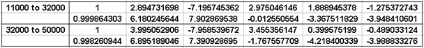 For each altitude range, the first row contains the numerator
polynomial coefficients and the second row the denominator polynomial coefficients.
For each altitude range, the first row contains the numerator
polynomial coefficients and the second row the denominator polynomial coefficients.
For both
altitude ranges, the rms error between the standard atmosphere values and the
approximation was 0.10%. For the lower altitude range the maximum error was
0.23%. For the higher range the maximum error was 0.27%.
Extending the Standard Atmosphere
The spreadsheet to be described in Chapter 7
is employed for modeling at much higher altitudes than 1,000 km. An extension
of the US standard has been devised by the writer for its use.
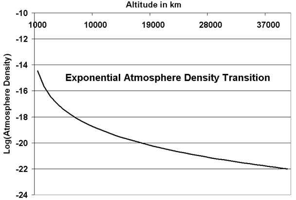
Since the atmosphere does extend above 1,000 km, an exponential extension is
chosen to match the 1976 US standard's density at 1,000 km and fall to the value
1E-22 at an arbitrarily chosen altitude of 40,000 km. For greater altitudes the
density remains at 1E-22.
A graph of the extension is shown next.
See
Wikipedia for further information on atmospheric densities.
For a distance comparison, the circumference of Earth is about 40,000 km.
For an application, consider that Geostationary satellites orbit at an altitude
of about 36,000 km.
The density at an altitude of 40,000 km may be much greater than 1E-22
but values are not available to this writer. What has been accomplished is a smooth
transition in density as altitude exceeds 1,000 km.
Having the need for a macro to provide the density values and having the plan to
provide a web based calculator for the viewer equivalent to the spread sheet, lead
to the decision to include all of the calculation needs of the spreadsheet in a
single macro. Then, assisting the viewer in creating his own spreadsheet by making
the macro and instructions for its use available for downloading. With this
process it becomes unnecessary for the user to type long mathematical expressions
into spreadsheet cells.
There is a calculation difference between the spreadsheet macro and the web-based
calculator.
The former employs single precision floating point arithmetic and the later double
precision. This was done to test the need for increased precision. The improvement afforded by double precision was judged as not very significant.
The Excel workbook consists of three named sheets:
Par contains
the parameter table,
Tab contains the data table and
Graph
contains the graphs.
There are five versions of the parameter table as it is changed by the macro to
suit each of 5 types of experiment, Expandable Balloons, Pressurized Balloons, Falling
Bodies, Vertical Projectiles, and Ballistics. See an example next:
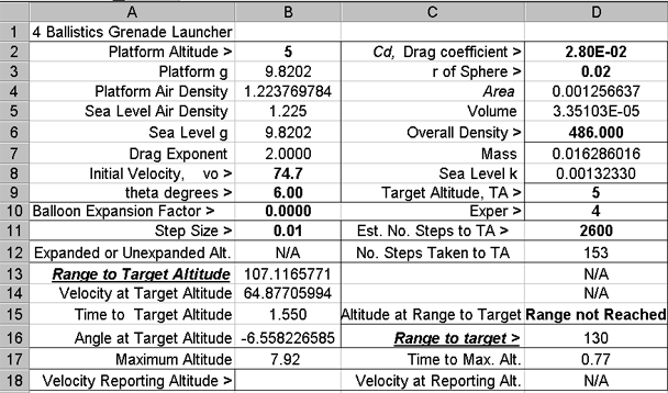
The five types are represented by a value 0 through 4 placed in cell D10.
The other inputs and outputs to the table will be described as the need arises.
A few lines of the Tab sheet are shown next:
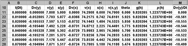
This table is not often used since most outputs of interest are extracted from it
and provided in the Par sheet. Note that rows 12 through 21 have been hidden
from view. This is because they contain components that are used to calculate
the first step that is shown in row 22. The reason for this special treatment
will be described later.
The columns from left to right contain - the time in seconds - the increment to
the velocity in the vertical direction - the vertical velocity - the altitude in
metres - the increment to the velocity in the horizontal direction - the horizontal
velocity - the horizontal distance - the combined vertical and horizontal velocity
- the travel angle of the object - the acceleration of gravity at the altitude -
the atmospheric density at the altitude - the acceleration of the body in the vertical
direction.
The spreadsheet and the calculator employ the same data table and parameter table
format.
Newton and Gravity Revisited
See Newton's law of universal gravitation
for an excellent discourse on this topic.
In Newton's theory of universal gravitation a point mass attracts another point
mass with a force that is proportional to the product of the two masses and inversely
proportional to the square of the distance between the point masses. That
is:
F = (G * m
1* m
2)/
d
2
The gravitational pull of a finite size spherical object with uniform density, is
as if it were a point mass at the sphere's centre, for regions exterior to the sphere.
Although untrue, the gravitational pull of the Earth is often modeled as being
the same for all points that are equally distant from the centre of the Earth.
Such a model would be expected to become more realistic as that distance increased.
The gravitational force is extremely weak. We don't notice it as we walk close
to other people
or near to heavy objects. Attempts to measure the gravitational constant G began with Henry Cavendish in ~ 1798. A history of its measurement and methods
can be found at
Gravitational constant.
The mass of the Earth, M, is no better known than is G. (Each is known
to about 1 part in 7000.) See
Standard gravitational parameter.
The value of product G*M, the standard gravitational parameter, is very much better
known, to ~ 1 part in 500,000,000. G*M = 398,600.4418 km
3s
-2.
For convenience, convert to units of m
3s
-2 to get G*M = 398,600.4418E09
m
3s
-2.
For an object with mass m that is outside the Earth and is d metres from its centre,
the gravitational force
on the mass is: F = G*M* m/d^2. That is, the acceleration of the object
is g = G*M/d^2. The radius of the Earth is about 6.37101E06 metres. Carrying
out the arithmetic for the surface gravity, the result is g ~= 9.82022.
The experienced value of g is affected by the Earth's equatorial bulge. (The Earth's
radius is greater at the equator than at the poles.)
Local variations in the terrain and in the subsurface have their effects.
The position of the moon has its effect.
Nonetheless, the value of g at sea level is only about 0.5% less at the equator
than at the poles.
At 80 km above sea level, g is about 0.975 of its sea level value. At 400 km above
sea level, g is about 0.885 of its sea level value.
The variation of g with altitude is incorporated into both the spreadsheet and the
web-based calculator.
Next
We illustrate a use of the calculator and further explore its features.