Background of Hands-On Math
Data Fitting - Curve Fitting - Interpolation
-Approximation - Maximizing - Minimizing - Optimization - Solving
Common Elements of Data and Curve Fitting, Approximation
and Optimization, Maximization and Minimization.
Data and Curve Fitting, Approximation, and Optimization are mathematical procedures.
They all employ numerical representations of: an Initial
State, Objectives
to be achieved, Controllables
that can be adjusted to reduce error, a
Current State or result that can be compared
with the objectives to produce a Current Error, and a Strategy
or strategies to find successive values for the controllables that reduce error.
Maximization and Minimization Procedures also employ numerical
representations of Initial State, Controllables, Current State and Strategy but
differ in that the Objective(s), and hence the Error(s), is(are) not usually defined by
fixed numerical values.
Sometimes a tentative numerical objective is provided as a large or small value
that can be compared with a Current State to produce, over some iterations, a least
achievable numerical Error. Although Excel's Solver is equipped to find Max, Min
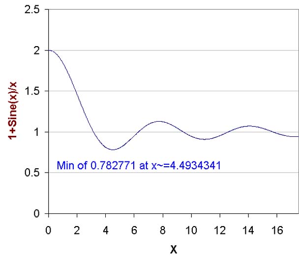
and Equals as objectives, the tentative objective technique can be illustrated with a simple example,
the minimum of (1+sinx/x). A graph of this function and the value of its minimum are shown next:
As Excel cannot readily find values for this function at x = 0, provide Solver with
a constraint such as x > = 0.0000001.
Now provide Solver with the tentative objective of setting the value of the function to, for
example, -1,000,000,000.
Set x to an initial value of 1.0 and start Solver. Solver will complain that
it was unable to reach a feasible solution. Notwithstanding the complaint it will
have found a somewhat inaccurate value for x quite close to the value for the location
of the actual minimum, for example, 4.49330.
The user may now choose an objective only slightly smaller than the minimum, e.g.
0.782 and Solver finds the value for x as 4.4934341 i.e. in agreement with the value
it would find if set up to locate a minimum rather than being set up to meet an objective.
Linear and Non-Linear
Gauss
is credited with being
first, in 1795 at age 18, to find the "Linear Least Squares" method that he used for fitting observations
that contain observational errors. Linear implies that the parameters of a model
are linearly combined. When this is so, a closed form of solution can
be found, not necessarily, but often in the form of polynomial coefficients. When the application is
non-linear, iterative procedures are employed.
Gauss Applied Linear Least Squares to Predicting
the Orbit of Ceres
Ceres, a new asteroid, was discovered on January 1, 1801 and tracked for 40 days
at which time it was lost in the Sun's glare.
At the age of 24, Gauss employed Linear
Least Squares to estimate and project the orbit of Ceres so that it could be located
when it emerged from behind the Sun.
In 1829, Gauss was able to show that a least-square estimator was the best linear
unbiased estimator of the polynomial coefficients when the measurements being fitted
had uncorrelated, equal variance, zero-mean errors - all properties that might
be expected of careful human measurements. This is the reason that the Least
Squares
representation of error is used when observational data is to be fitted with a curve.
Least Squares minimization can also be thought of as a neat way of smoothing data that
has a large error component
Fitting a Curve with a Curve, Approximation
There are cases where the curve to be fitted is not the result of noisy physical
measurements that require smoothing and instead is the result of labour-intensive
calculation.
What is then desired is a more simple expression for a range of the calculated curve.
In this case the objective is to find a new curve that is less complex to calculate
and which, although not an exact fit, is satisfactory in some sense.
This is a case where the data to be fitted is regarded as exact and,
for the sake of reduced calculation effort, we are willing to accept a less precise
representation.
As an example, the A and B coefficients of the function Y = A * X + B / X
are now chosen, using Solver, to fit the calculated function Y = X ^ 0.5 which
has been calculated at 201 points from X = 0.25 to X = 2.25.
(The fitting function has been chosen rather arbitrarily only to show the
effect of using two alternatives to Least Squares.)
Name the 201 values of calculated Y, C1 through C201. Name the corresponding
201 values that will be found for function Y, F1 through F201. Postulate errors,
E1 through E201, which can be found for each point by comparing
the corresponding Ci and Fi values. There are many possible ways of forming
the Ei values.
Least Squares would set Ei = (Ci-Fi)^2 and Solver would be used to choose A and
B so as to minimize the sum of the 201 Ei values.
Sometimes it is of interest to chose Ei as Abs(Ci-Fi) so as to minimize Absolute
Error rather than squared error.
At other times it is Relative Error that is important. We would might use
either Ei = abs( Fi / Ci - 1) or Ei = ( Fi / Ci - 1) ^2.
In addition to such choices, some users would prefer to minimize the greatest of
the Ei rather than their sum, MiniMax. Perhaps there are other users who would prefer
to make the two largest errors as equal and as small as possible. Who knows?
To illustrate the effects that can occur with choice of the error criterion, Solver
was employed to fit the list of square roots using MiniMax for both the Absolute
Error criterion and the Relative Error criterion as seen next:

For the Minimum Absolute Error fit, blue, the maximum error is seen to occur at
both the largest and smallest X values. This results in a comparatively high relative
error for X near 0.25.
For the Minimum Relative Error fit, red, the maximum error is seen to occur at the
largest X value.
Which of these two fits would you prefer?
When the object is solely a close fit, greatest interest may be on using the criterion
and other strategy that would provide a satisfactory fit with the least expenditure
of calculation time. That is a subject outside of the scope of Hands-On Math.
Interpolation
Note in the foregoing example of curve fitting that it was incidental that the fitting
expression interpolated the 201-point list. There can be occasions when the
interpolation aspect of curve fitting is the primary objective although the fit
remains important.
Optimization - Minimization - Maximization
Curve fitting can be described as having the objective of fitting a
curve with minimum error. However there are times when the objective is not a curve
but is instead a combination of disparate items such as fuel efficiency, dollar cost and size and the objective is to minimize a weighted combination of
such items.
If the objective were to maximize the ratio of size to dollar cost for a given fuel
efficiency we would think of the problem as one where the optimum was found when
that ratio was largest.
Methods for minimization and maximization differ little. A large quantity becomes
small when; instead, its inverse is the objective.
The term Optimization is most often employed when the objective combines
disparate items whether or not the application is one of maximization or minimization.
Optimization
When the objective function is a weighted sum of disparate items, such as are found
in modeling
a projectile aiming at a target. Example items are: the
time that a position is reached, the
angle of approach at that time and the
velocity at that time. The controllables may also be disparate
such as Charge, Elevation, and Azimuth.
If the projectile were a grenade aiming at a moving target then the time and angle of approach might be given
most weight. If it were a shell aiming at a stationary
target then velocity and angle of approach might be weighted
most.
When the controllables are disparate. The sensitivities of the weighted objective to the
controllables will be disparate and must be separately weighted in adjusting the
controllables. Otherwise one or more of the sensitivities could be too small to
affect the optimization or so large as to weaken or destroy convergence.
This situation can be looked after by the user intervening initially to set the
weights and from time to time intervening to adjust the weights. In come cases
means can be found to automatically adapt the sensitivity weights as iteration progresses.
Numerical Differentiation
Just as numerical integration resides at the core of the numerical solution of differential
equations, numerical differentiation to determine sensitivities is the core procedure of numerical optimization.
The methods to be employed could be absolute or relative, e.g., a controllable could
be changed by a small constant amount such as 0.0001 or by 0.01%, the former being
a concern when the value of the controllable is both very large such as 1,000,000,000,000
and very small such as 0.000,000,000,001, the latter creating concerns when
the value of the controllable is at or near zero.
There are two-point, three-point and even five-point differentiation methods. There is Differential
Quadrature, which uses weighted sums of function values. There are methods based
on Splines, methods based on Taylor series, and other methods can
be devised or found.
This writer tends to favour the use of forms of relative error in situations where
the controllable does not take on the value of zero and the computer being used
is efficient at division.
Solving
Sets of linear and non-linear equations or a mixture of both may be solved iteratively
with an optimization routine such as Solver.
This ability to solve can be looked upon more broadly as an ability to estimate
or infer the cause of an observed effect.
Could observation of the tides, at a position on the Earth, and over a period of
months become a basis for any inferences about our Moon, its orbit or about properties
of Earth?