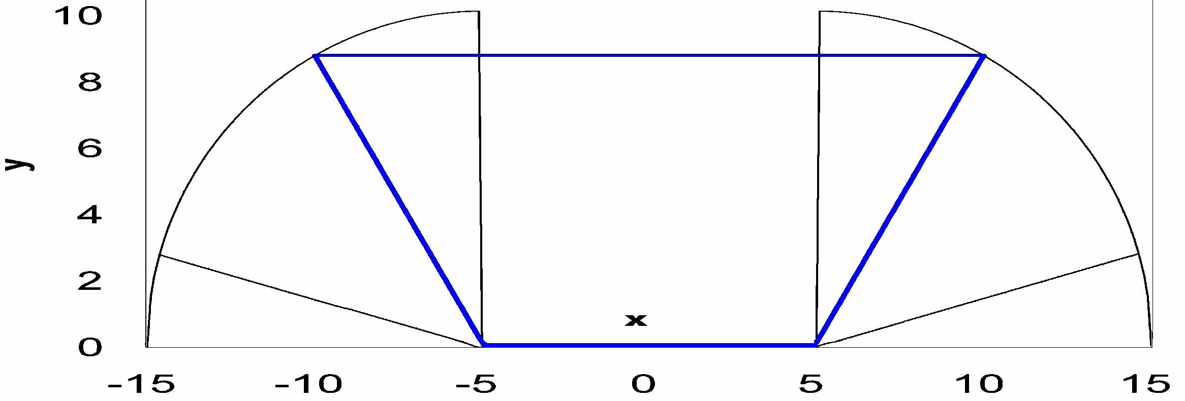
Start with a 30 cm wide, long
flat piece of sheet metal,
lying in the horizontal plane. Make sharp bends at 10 cm in from
each of the left and right edges as is seen in the diagram following. Bend
each side up the same amount.
There must be some bend that will provide the most trough volume. If so, what will
be the height and width of the trough?
To answer the question we require an expression that relates a dimension of the
bent section to the volume, or equivalently, to the area of the trough's cross section.
We decide to relate the amount of bend to the x coordinate of the tip of the bend
on the right. Its range is 5cm. through 15 cm. The y coordinate of the tip
of the bend is given by:
The area of the trough a is given by a = y*(10+x). A short spreadsheet table is used to verify our assumption that there is an optimum bend
and if so to localize it. We start with x = 5 cm. and increment it in amounts
of 2 cm. as seen next.
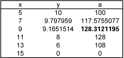
Without proceeding further one could choose a bend where x and y were both slightly
over 9 cm, but then we would miss the fun part.
Use a spreadsheet.
Start at x = 7 cm, use initial small steps, ∆x =
0.1, and hunt for the maximum by reversing step
direction with smaller step size, i.e., ∆x/2, whenever the area is seen to be decreasing
with the current step size.
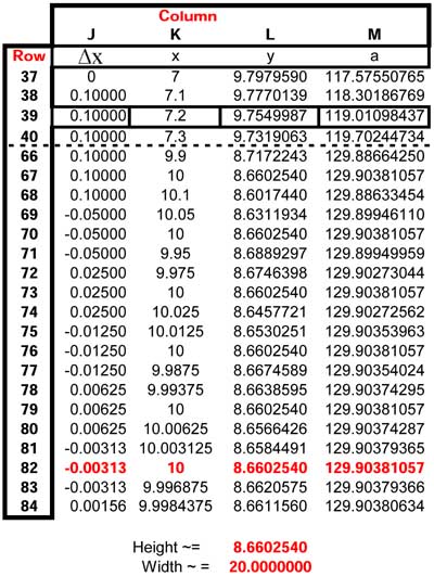
Only the more interesting steps are shown in the table. Notice that the process
seems to be homing in on x = 10 and therefore choose that value as optimum.
Click the cell addresses following to view the cell expressions.
What about the choice of positioning the bends at 10 cm from each edge? Why
don't you use a spreadsheet to see if there is a choice that will provide more
area?
In some situations we search for a minimum. How would the search algorithm
change?
Try Polar Coordinates
When a position in a plane is referenced by its distance, r, from a point
of origin and its angular offset, θ, from a straight line that passes through
that origin, it is being referenced by its polar coordinates r, θ.
Polar coordinates are often most convenient when the problem at hand has some
angular symmetry.
When the reference line coincides with the x axis and θ is taken to increase positively
with counter clockwise rotation, then one can convert to rectangular coordinates
using x = r*cos(θ), y = r*sin(θ). The inverse expressions are θ = arccos(x/r)
and θ = arcsin(y/r). (Sometimes arc is abbreviated to a.)
The unit that is often used for θ is the radian although the degree is sometimes
convenient. There are 2π radians to a single 360o
rotation around an origin.
Return now to the design of the eave trough. The right 10 cm. flap of the sheet
metal, is bent upward by an angle θ from the angle 0 radians to some angle < π / 2 radians. The height h of the trough is 10*sinθ.
Its width
w is 10*cosθ +10 +10*cosθ. Its area a
is 100*sinθ*(1+cosθ).
A rough calculation using steps of 0.25 radians finds a maximum of about 130 cm2 near θ = 1.
A more precise maximum is then found using an adaptive step size with θ increasing
from 0.75
radians. In this case the change in area, Δa was calculated so that
calculation could be terminated when Δa reached ~10-8.
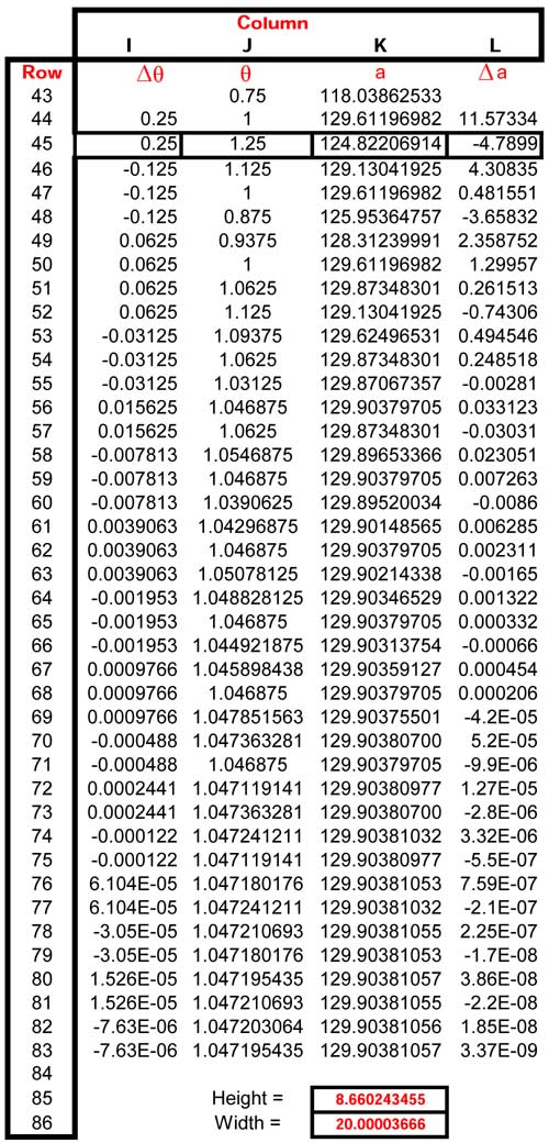
The expressions for the outlined cells in rows 45, 85, and 86 can be seen by clicking
the cell addresses that follow.
Whether to employ polar or rectangular coordinates in this optimization problem
appears to be six of one and a half dozen of the other.
Next
Optimization and Approximation are closely related topics. Approximation with sinusoids
is explored next.