Chapter 3
Exploring Spreadsheet Integration -
Multiple Integrations - Larger Numbers of Steps
Performance After a Series of Integrations
The need for multiple integrations, integrating the results of integration, occurs
in content problems that we have in our space of three physical dimensions. The need
also occurs in theoretical investigations that may involve a great many dimensions, see next.

Schlafli
, 1814 - 1895, a Swiss mathematician is credited with developing the Euclidean geometry
of n dimensions. He introduced the notion of a group of n coordinate values
representing a point in an n space. He introduced polytopes as higher dimensional
analogues of polygons and polyhedra.
In a modern computer or communications context,
all of the 2^64 possible 64-bit binary words can be described as the coordinates of
the vertices of a cube in 64-dimensions.
While
Euclid
~325 BC -~265 BC, proved that there are exactly five regular solids in a three-dimensional
space, Schlafli proved that there are exactly six in four dimensions and exactly
3 in five and higher dimensions.
Schlafli made an important contribution
to non-Euclidean geometry by proposing that spherical 3-dimensional space could
be regarded as the surface of a hyper sphere in Euclidian 4-dimensional space.
As numerical integration provides only an approximation to a true integration, one
can expect the result of successive such integrations to worsen in comparison with
the true result. To test this expectation the true result of successive integrations
must be accurately known. Since the integration of sinusoids results in sinusoids
the sinusoid was chosen as the integrand. A simple numerical integration process
was chosen for study.
It was decided first to employ the 4-point Gaussian Integrator to integrate sin(x). This emulates the use of a very precise DA Input Table.
Then, next,
to follow with a sequence of integrators each employing rectangular quadrature.
Each integration employed 1000 equal steps in the range x = 0 to x = 2 * π.
The "Input Table" section is shown next.
The expressions contained in the outlined cells, foregoing,
can be seen by clicking their addresses next.
B1 contains the step size and I2 contains the maximum
integration error. F7 contains the weighted evaluations of sin(x) at the 4
Gaussian points multiplied by the step size.
G7 shows a step of the accumulation given the initial value of -1 in G6. This is
expected to be, closely, the negative cosine of x, A7.
The negative cosines of x are calculated in column H and can be seen to agree quite
closely with the accumulator values, the results of 4-point Gaussian Quadrature.
The results for some of the calculation steps of the first
two of 61 successive rectangular quadrature integrators are shown next. The maximum
errors are shown in cells M2 and G2.

The expressions contained in the outlined cells, foregoing, are available next.
The essential difference from the Input Table that receives
its input from the sine function is that the first of these integrators receives
its input, Dy, from the accumulator of the Input Table and the second of these integrators
receives its input from the accumulator of the first integrator.
Each of the remaining 59 integrators is coupled to its predecessor in the same manner.
Note that the maximum error at the accumulator of these integrators seems to increase
as the number of integration stages increases.
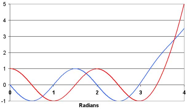
The final two integrators of the sequence are shown next.

Note that the maximum errors have increased but remain
quite tolerable. This may be better grasped from the chart following:
 The eye would not be able distinguish the foregoing plots
from -cos(x) and -sin(x).
The eye would not be able distinguish the foregoing plots
from -cos(x) and -sin(x).
The behaviour of the maximum error versus the stage of integration can be of interest.
The maximum errors have been collected into an array with four columns so that all
integration outputs that are nominally the same function occur in the same column.
That array follows:
Note that the maximum errors seem to settle to values
that appear to be identical for all subsequent integrations that result in the same
function. This may not be true. The foregoing figure shows 16 decimal digits
and after stage 7 there are four leading zeros. With Excel's arithmetic there
can be no more than 16 significant digits. This suggests that 4 more decimal
digits could be shown with likely little significance to be attached to the last
digit. That array follows:
It is now seen that after stage 30 of integration the
maximum errors remain constant and, as one might expect, do not depend on the sign
of the function. The constancy achieved by the maximum errors is a remarkable result!
What is the effect of reducing step size? With 1/2 or 1/4 of the step size, the values
of the functions will still cover the range 0 to 1. See the effect on
maximum error of half the step size next.
 The maximum rectangular quadrature error in the stabilized
zone has been reduced by a factor of about 10.
The maximum rectangular quadrature error in the stabilized
zone has been reduced by a factor of about 10.
Next, the step size is again halved.

The rectangular integration maximum errors in the stabilized zone have again decreased by approximately an order of magnitude.
Notice that the reduction of step size has resulted in earlier stage stabilization
of the maximum errors.
Lag
The output of a numerical integrator can only be supplied to its input at or later
than the next available input calculation step.
The same is true for an electronic integrator such as an
Op Amp in that electrical transmission time, albeit very small, is required before its
output can be applied to its input.
There is a similar effect, a very small delay in the mechanical transmission of
force, when the output of a mechanical integrator is returned to its input.
In numerical integration the size of the first step can be made quite small relative
to the size of the steps that follow should a smaller initial lag be desired.
Feedback
Observe that the Table Input integrator that provides
input to the first rectangular integrator may not be necessary. Its output
function, -cos(x), also exists at the output of stages 4, 8, 12, ........,
60.
Although it might seem a lot like lifting oneself up by one's own bootstraps, it
will be interesting to substitute one of these for the Table Input integrator. (Creating
a feedback connection.)
Feeding the output of stage 60 back as the input to stage 1 is accomplished by changing
cell J8 from =(G7+G8)/2*$B$1 to =(IM6+IM7)/2*$B$1, and changing subsequent cells
in column J accordingly. Cell J7 was set to 0 and is to be considered later
in this topic. The outputs of the
60th and 61st
integrators are shown next.

Surprise! As far as the eye can tell, both are sinusoids.
The maximum errors are shown next.

More and smaller steps
A general procedure to lessen error is to simply employ more steps and make them
small enough to satisfy ones own precision needs. Next, the step size is reduced
by a factor of four and the number of steps is increased by the same factor.
This change has reduced the worst error, stage 1, by a factor of about 4.
The worst of these occurs with the first three integrators. Perhaps this could be ameliorated by selecting a value for cell J7, a cell that had been set to 0.
Now employ Solver to choose J7 to minimize the maximum error of any the first 3
integrators. This choice was made in order to reduce the possibility that other
errors might grow if just the one error were minimized. The result follows:

The new value for cell J7 is: -0.0001964024032407, curiously, about equal in magnitude to the new maximum error of the first
integrator. This
result may be interesting but, to continue exploration, restore J7 to the value 0.
A Sign Change
With a change of sign, a stage that has a + cos(x) output can be fed back to the
first integrator. (Some would call this Negative Feedback as opposed to Positive
Feedback as used heretofore.)
The 58th stage will
be fed back to illustrate.
Also, the value for J7 will again be chosen to minimize
the maximum error of the first three integrators. The result is seen next.
This case required exactly the same value for cell J7 as did the previous case and
provides identical maximum errors.
Although the foregoing adjustments of J7 did lessen maximum error, the process, although
interesting, does not seem very general in its application, although it could possibly
be of use at times. Accordingly, the value 0 is restored to cell
J7
A general procedure to lessen error is to employ more steps and make them small
enough to satisfy ones own precision needs.
Increasing the Number of Steps with a Fixed Step
Size
How does error behave as the number of steps
is increased for a given step size? To examine this question, the 6th
stage of the foregoing example was fed back to the input of the first stage and
the number of steps was increased by a factor of four. There was no change to step
size.
Maximum error was then calculated for each integrator output for 4 equal ranges
of x, 0 to π, π to 2π, 2π to 3π, and 3π to 4π, every half cycle of the
sinusoids. These errors are shown next.
The sinusoids from the first two integrators are plotted next.
Should one desire more precision, the step size can be
reduced further and more steps employed.
The viewer might wonder whether variable step size might be used to improve precision. Don't know? Give it a try!
The spreadsheet has been shown to be an excellent tool for the exploration of fed
back and non-fed back systems of integrators and their associated parameters, albeit
in a very particular situation.
Subsequent topics will delve further into aspects of applying the spreadsheet integrator.