Chapter 7

Three Dimensional Modeling -The Spreadsheet

Documentation

This spreadsheet is, in the main, a large macro written in the Visual Basic language. Rather than describe the spreadsheet in Visual Basic terms, the writers have chosen to employ a largely mathematical description.

The applications of the worksheets are to determine trajectories in three dimensions for orbiting (and sub-orbiting) objects. Newton’s inverse square law of gravitational attraction, buoyancy and atmospheric resistance are accounted for in the equations.

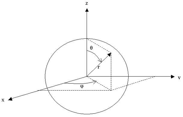
The coordinate system is xyz. The origin is such that the central body being orbited is assumed to be spherical with its centre fixed at the origin of the xyz system with the z-axis emerging from the north pole of the sphere. The xyz coordinates are absolutely fixed with respect to the universe.

In the case of the Earth, the central body rotates on its axis once per sidereal day. A point located on or near Earth is specified by fixed Latitude, Longitude, and Altitude coordinates. In terms of the xyz coordinate system, points attached to Earth have their xy coordinates constantly changing due to rotation about the z-axis.

The atmosphere is assumed to rotate with the Earth. The model is set up such that the launch point is in the xz plane at t = 0 (the time of launch), irrespective of where the point is located on Earth.

Worksheets

There are four worksheets, Paris, Geo, Elliptic, and Planet, each intended for different modeling situations.

Paris

This sheet is intended for sub-orbits near Earth where atmosphere resistance is at play. Inputs include the location of the launch point. Outputs include the impact point and its range and bearing from the launch point. It is assumed that the launcher is fixed to the earth.

Geo

Used to study geosynchronous orbits that are strictly along the equator of the body being orbited.

Elliptic

Used to study arbitrary orbits.

Planet

Intended for use in determining the trajectory for any planet.  A site that provides data for planet orbits can be seen here.

Charts of orbits are the orbits projected on the xy plane.  Highly inclined orbits will usually look artificially elliptical.

Input Parameters

The same set of parameters, more or less, is provided for all the sheets. The exact set of parameters, their interpretation and wording, changes from sheet to sheet.

Latitude, Longitude, and Altitude are Earth based coordinates of a launch point.  For a satellite launch, Latitude and Longitude are values projected down to earth's sea level.

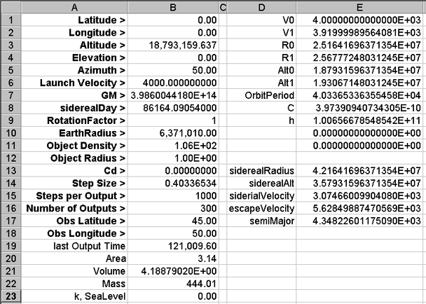
See the following parameters for the Elliptic sheet as an example.



Latitude

This is the latitude, in degrees, of the launch point as measured on the earth. On the planet sheet this parameter is used to specify the initial location above/below the orbit plane that the planet has at t = 0. For satellites on the Geo sheet, Latitude is forced to 0.

Longitude

This is the longitude, in degrees, of the launch point as measured on the earth. East is positive and West is negative.  The launch point is always aligned with the xz plane at t = 0.

Altitude

On the Planet sheet, this parameter is Distance and represents the centre-to-centre distance between the sun and the planet. For the other sheets, this is the altitude of the launch point.  Altitude is zero at sea level on earth.

At time t = 0 a launch point is in the xz plane so the initial x, y, z, r, θ, φ  of the object are:

          r  = earthRadius + Altitude
          θ  = 90 - Latitude (degrees)
          φ  = 0
          x  = (earthRadius + Altitude) * cos(Latitude)
          y  = 0
          z  = (earthRadius + Altitude) * sin(Latitude)

Elevation

This is the launch point elevation in degrees, the angle above the local horizontal or tangent plane that the launch barrel is pointing.  The meaning is similar for satellite launches; elevation is zero if the object is launched in the tangent plane.  For satellites on the Geo sheet elevation is forced to zero.

Azimuth

This is the number of degrees from north the launch barrel is pointed, as measured in the tangent plane.  On Earth this would be called the compass bearing.  East is 90 degrees and so on.

Launch Velocity

This is the initial velocity of the object in meters per second.  For a cannon or other launch device attached to the Earth, the Earth's spin on the z-axis imparts an easterly velocity to any launched object. The appropriate velocity is provided by the software as determined from the latitude of the launch site.

After launch, the object is subjected to the same orbital physics as are satellites and planets.  The velocity of an orbiting object is measured with respect to the xyz coordinate system.  Except for the Paris sheet, the launch is assumed to occur from a platform that is stationary with respect to the xyz coordinates.

G*M

The Standard Gravitational Parameter.

For Earth G*M ~= 398,600,441,800,000 metres^3/second^2.
For our Sun G*M ~= 132,712,440,018,000,000,000 metres^3/second^2.

Sidereal Day

This is the rotation period of the Earth in seconds, not used on the Planet sheet. It is used to calculate the longitude of an object at a given time. The longitude is needed to calculate the arc distance and bearing from launch point to object.  If the objects coordinates are x, y, z then:

      Object_r = sqrt(x^2 + y^2 +z^2)
      Object_θ  =atan(z / r)
      Object_φ  =atan(y / x)

Since φ corresponds to Longitude and φ = 0 for the launch point at t = 0, then at time t

      Launch_φ = (2 * π * t) / SiderialDay

The Longitude of the object at any t, x, y, z, is:
        
Object_Longitude = atan(y / x) - (2 * π  * t ) / SiderialDay + Longitude

Also, Object_Latitude =  π / 2 - Object_θ 
                                      = π / 2 - atan(z / r)

Rotation Factor

The value zero turns off earth's rotation, the value one turns it on. This could be used to demonstrate the effect of Coriolis.

Earth Radius

We usually employ a radius of 6,371,010.00 metres.

Object Density, Object Radius, Cd

These parameters are the same as described in Chapter 3 and Chapter 6. For a discussion of Cd, see Chapter 6 "The Drag Coefficient".

In Chapter 3 we took buoyancy into account as a modification to g in the differential equation. That was because buoyancy creates a force that is opposite to gravity: One may think of an effective or buoyant mass mb for an object with mass m where: mb = m * (1 - pfluid / pobject).  Under gravity the object will fall if its density is greater than that of the fluid and rise if less.

Step Size

This is the integration interval in seconds.

Steps Per Output

This is the number of integration steps from one output row to the next.  Use 1 to get one output for each integration step.

Number of Outputs

This is the total number of rows of output. If Outputs were 1,000 and Steps were 1,000 then there would be 1,000,000 integration steps.

Last Output Time

The value in this cell is Step size * Steps Per Output * Number of Outputs.

Area, Volume, Mass, k Sea Level

These are the same as in previous topics.

Obs Latitude

On the Elliptic sheet.  This is the latitude of an observer on earth, in degrees. North is positive.

Obs Longitude

On the Elliptic sheet. This is the longitude of an observer on earth, in degrees. East is positive.

Analytic Outputs

These are seen in column D and were described in the preceding topic.

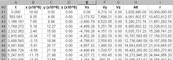
The Output Table

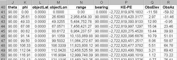
Some rows from the output table for the Elliptic sheet are shown next, in two sections.

The output needs of the four sheets differ, just as their input needs differ.  Some columns are required on one sheet and not on another.

All sheets show the object coordinates with time: t, x, y, z as well as r, θ, φ.  Distances are in metres for the Paris sheet, megametres for Satellites, and gigametres for planets.

On the Paris, Geo, and Elliptic sheets there are also columns for:

Alt = r - earthRadius
ObjectLat = sub-point on Earth latitude of object
ObjectLon = sub-point on Earth longitude of object
Range = distance from launch sub-point and to object sub-point as an arc distance
Bearing = azimuth angle from launch sub-point to object sub-point measured clockwise from North.
KE-PE is kinetic energy less gravitational potential energy:
    = mass * (Vx^2 + Vy^2 + Vz^2)  / 2 - GM * mass / r
    At escape velocity KE-PE is zero.

The Elliptic sheet has two additional output columns:
Obs Elevation is the elevation the observer sees between his horizon and the object in orbit, in degrees.
Obs Az is the azimuth the observer sees between his north compass point and the object in orbit, in degrees, measured in his tangent plane

Integration Routine for Macro

Overall, the macro that processes the spreadsheets is organized as follows:

   Calculation()
    Initialize (determine all required globals, including standard atmosphere model)

    GetInputs()
   (get the configured parameters for the simulation)

    OutputAnalytics()
    (analytic calculation)

    Integrate() 
     (There is a choice of employing a first or a second order integration process. The second order process is further discussed subsequently. Both processes include writing individual rows of output at prescribed intervals of the integration process)

    OutputResults()
    (this includes drawing charts according to output rows derived by Integrate())

    End

Apart from second order integration, the routines in the macro use straightforward spreadsheet processes to obtain and present data. Formulas used for analytic calculations are covered elsewhere.

The integrate subroutine is best described with psuedo-code. The syntax used corresponds to Excel Basic:

   Integrate()

   ' set up the initial values for variables according to configured inputs
   If (ActiveSheet.Name = "Planet") Then
      r = launchAlt    ' the entered value is center-center distance
   Else
      r = earthRadius + launchAlt
   End If
   Theta = Pi / 2# - launchLat
    phi = 0
    x = r * Sin(Theta) * Cos(phi) 
    y = r * Sin(Theta) * Sin(phi) 
    z = r * Cos(Theta) 
    Vr = launchVelocity * Sin(launchElev) 
    Vtheta = -launchVelocity * Cos(launchElev) * Cos(launchAz) 
    ' for the Paris worksheet, the object is launched from a cannon that is rotating 
    ' with the earth, so imparts an additional phi velocity to the object 
    If (ActiveSheet.Name = "Paris") Then 
       Vphi = launchVelocity * Cos(launchElev) * Sin(launchAz) + factor * 2 * Pi * r * Cos(launchLat) / siderealDay 
    Else
   Vphi = launchVelocity * Cos(launchElev) * Sin(launchAz) 
    End If 
    ' Resolve the spherical V into Cartesian V
    Vx = Vr * Sin(Theta) * Cos(phi) + Vtheta * Cos(Theta) * Cos(phi) - Vphi * Sin(phi) 
    Vy = Vr * Sin(Theta) * Sin(phi) + Vtheta * Cos(Theta) * Sin(phi) + Vphi * Cos(phi) 
    Vz = Vr * Cos(Theta) - Vtheta * Sin(Theta) 

    While (i <= lastStep)
       r = Sqr(x ^ 2 + y ^ 2 + z ^ 2) 
       r3 = r ^ 3 
       Theta = thetaFromXYZ(x, y, z) 
       phi = phiFromXYZ(x, y, z) 
       If (stepsSinceLastOutput >= stepsPerOutput) Then 
          ' each sheet has its own layout for output, call respective subroutine 
          If (ActiveSheet.Name = "Paris") Then 
             OutputRowParis 
          ElseIf (ActiveSheet.Name = "Geo") Then 
             OutputRowGeo 
          ElseIf (ActiveSheet.Name = "Elliptic") Then 
             OutputRowElliptic 
          ElseIf (ActiveSheet.Name = "Planet") Then 
             OutputRowPlanet 
          End If
          stepsSinceLastOutput = 0 
       End If
    ' Calculate the forces acting on the object at this time 
    ' For the Paris sheet, the following set of equations assume the Earth drags 
    ' the atmosphere along totally. At earth's surface 
    ' the atmosphere moves at the same speed as the ground, etc. 
    If (ActiveSheet.Name = "Paris") Then 
        Wr = 0 
        Wtheta = 0 
        Wphi = factor * 2# * Pi * r * Cos(launchLat) / siderealDay 
        Wx = Wr * Sin(Theta) * Cos(phi) + Wtheta * Cos(Theta) * Cos(phi) - Wphi * Sin(phi) 
        Wy = Wr * Sin(Theta) * Sin(phi) + Wtheta * Cos(Theta) * Sin(phi) + Wphi * Cos(phi) 
        Wz = Wr * Cos(Theta) - Wtheta * Sin(Theta) 
    Else 
        Wx = 0 
        Wy = 0 
        Wz = 0 
    End If 
    ' total force on the projectile is sum of buoyancy, air friction, gravity. 
    ' buoyancy factor (BF) is radial, friction factor (F) is in opposite 
    ' direction of velocity. 
    ' BFr, FFv group common factors to avoid duplicate multiplications 
    Sy(row) = r - earthRadius 
    Atmosdensity ' update ph(row) for this value of Sy(row) 
    BFr = GM * (1 - ph(row) / Density) / r3 
    ' radial bouyance and gravity factor 
    FFv = Kay / 1.225 * ph(row) 
    FFx = FFv * (Vx - Wx) ^ 2 * Sgn(Vx - Wx) 
    FFy = FFv * (Vy - Wy) ^ 2 * Sgn(Vy - Wy) 
    FFz = FFv * (Vz - Wz) ^ 2 * Sgn(Vz - Wz) 
    ' get the current acceleration due to these forces 
    ' use second order update process ie 3*Fcurrent/2 - Aprevious/2 
    Ax = -(BFr * x + FFx) 
    Ay = -(BFr * y + FFy) 
    Az = -(BFr * z + FFz) 
    x = x + 0.5 * (3 * Vx - prevVx) * delta_t 
    y = y + 0.5 * (3 * Vy - prevVy) * delta_t 
    z = z + 0.5 * (3 * Vz - prevVz) * delta_t 
    ' done with using prevVi, so update them for next time through loop 
    prevVx = Vx 
    prevVy = Vy 
    prevVz = Vz 
    Vx = Vx + 0.5 * (3 * Ax - prevAx) * delta_t 
    Vy = Vy + 0.5 * (3 * Ay - prevAy) * delta_t 
    Vz = Vz + 0.5 * (3 * Az - prevAz) * delta_t 
    ' done with using prevAi, so update them for next time through loop 
    prevAx = Ax 
    prevAy = Ay 
    prevAz = Az 
    ' move to the next step and increment quantities accordingly 
    i = i + 1 
    ' for the first set of steps, time, t = t + smaller, dynamic time increments. 
    ' after that, time is determined by stepSize and i (= step number) 
    If (i > 10) Then 
        t = (i - 10) * stepSize 
        stepsSinceLastOutput = stepsSinceLastOutput + 1 
    ElseIf (i > 2) Then 
        smallStepSize = smallStepSize * 2 
        t = tPrev + smallStepSize 
    Else 
        t = tPrev + smallStepSize 
    End If 
    delta_t = t - tPrev 
    tPrev = t 
    Wend

End Sub ' Integrate

Second Order Integration

Many methods have been developed for numerical integration. Their many descriptions and applications are beyond the scope of this topic. The reader will find many sources of information on methods of numerical integration in mathematical texts and on the Internet. 

How do you measure the worth of an integration method?  When computation time is considered as important, a user would like to achieve a desired precision while using the least calculation time.  For a given problem class some methods will be better in this sense than others.  Our 3D spreadsheet macro provides the user with two choices, a first order process and a second order process.

The fundamental step in first order integration involves deriving a new quantity, such as velocity, by adding to the current velocity the product of acceleration and the time interval of the step. This first order process produces better results the more slowly the involved quantities change over time and the smaller the time interval of the step. 

Second order modeling may improve the process, especially where the quantities change with time but are well behaved, as in the motion of satellites around the earth.

To describe second order integration more precisely, let the time varying acceleration, velocity and position be represented by the symbols A(t), V(t), and R(t), respectively. At any particular step in the integration, the time t = t0, V(t0) and R(t0) are known because they are derived from the integration loop. The acceleration A(t0) is calculated from the velocity V(t0) which in turn has been calculated from the influences of gravity, buoyancy and atmospheric resistance on the object at position R(t0).

To obtain a second order estimate of the next value of velocity V (at time t1 = t0 + Dt where step size Dt  =  t1 - t0  =  t0 – t-1), we approximate V(t) with the first three terms of a  power series , around the current time, t0. This series is:

V(t) = V(t0) + C1 * (t – t0) + C2 * (t – t0)^2

, where C1 and C2 are constants that can to be found in the manner that follows.

Rearranging the foregoing expression and presuming that time dt is extremely small gives:

dV = V(t + dt ) - V(t)
      = V(t0) + C1 * (t + dt – t0) + C2 * (t + dt – t0)^2
       - V(t0) - C1 * (t – t0) - C2 * (t – t0)^2

Then expand the squared terms to provide:

dV = V(t0) + C1 * (t + dt – t0) + C2 * (t^2 + dt^2+ t0^2 +2t*dt -2*t*t0 -2*dt*t0)
- V(t0) - C1 * (t – t0) - C2 * (t^2 - 2 * t * t0 + t0^2)   then, presuming that C2*dt^2 is so small that it can be neglected and collecting terms obtain:

dV =  C1 *  dt  + 2 * C2 * (t -t0) * dt  or:

A(t) = dV/dt = C1 +2 * C2 * (t – t0)

Then at t = t0:

A(t0) = C1 + 2*C2 * (t0– t0)

That is:  C1 = A(t0)

At  t =  t-1

A( t-1) = C1 + 2 * C2  *  ( t-1– t0)  and since ( t-1– t0)  = -Dt

A( t-1) = A(t0) - 2 * C2  *  Dt  = Thus:

C2 = (A(t0) - A( t-1)) / (2*Dt )
          
The velocity model is:

V(t) = V(t0) + C1 * (t – t0) + C2 * (t – t0)^2     that, using the values for C1 and C2, becomes:

V(t) = V(t0)  + A(t0)  * (t – t0) + (A(t0)  – A(t-1)  / (2 *  Dt) * (t – t0)^2 

Setting t = t1 gives a second order estimate of velocity V(t1) as:

V(t1) = V(t0)  + A(t0)  * (t1 – t0) + (A(t0)  – A(t-1))  /  (2* Dt)  *  (t1 – t0)^2

and setting  (t1 – t0) = Dt we obtain:

V(t1)  = V(t0)  + A(t0) * Dt     +    (A(t0)  – A(t-1)) / 2 * Dt  or:

V(t1)  = V(t0)  + ( 3 *A(t0) – A(t-1))  * Dt /2

Which is the sought second order estimate for V(t), Note that A(t0) must be retained in memory to serve as A(t-1) in the next iteration.

We sometimes describe the process of estimating the next value as a prediction method.

Comparative Performances of First and Second Order Integration in Vacuum 

In the absence of an atmosphere the period of an orbit can be determined analytically with great accuracy. In exactly one period the xyz parameters should be identical to those at the beginning of the period.  This fact is used to compare the performance of integration methods and step sizes.

For the comparison we chose a body in an eccentric equatorial orbit with a minimum altitude of 100,000 m and maximum altitude of about 626,849 m.  The chosen period was 5500 s.

A chart showing the xyz parameters for this orbit at t = 0, and again at t = 5500 employing 1st order integration, red, and 2nd order integration, blue, each with three step sizes is shown next:



It can be observed that 2nd order integration with step size 0.55 s provides a more accurate result than does a step size of 0.000055 s when 1st order integration is employed.

Note that the derivation of a second order integration process for use when step size is not uniform is available from the Download tab on the upper row of tabs. As it provides a somewhat broader and more detailed view of numerical integration, the interested viewer may wish to consult it.

Second Order Integration in Atmosphere 

There are no analytic benchmarks for trajectories in atmosphere.  One method of determining a useful step size for a class of problem is to observe the convergence of trajectory characterization values, as step size is made smaller. This is the procedure now illustrated.  

For illustration we chose a body with a velocity that in vacuum would result in a circular equatorial Earth orbit at an altitude of 1,000 m with period of just over 5062 seconds.  In atmosphere it will be in a sub orbit and fall to the Earth The body was assigned a Cd of 2.0. Its xyz parameters and altitude at t = 40.49632755.... s were observed for a range of step sizes.  See the results next:



The accuracy required by the user might be to about the nearest metre in altitude. Noting that there is little and diminishing change in reported altitude taking place when step size is below ~0.005, then that or a slightly smaller step size could be chosen. 

Next

The use of a spreadsheet to find a complete orbit from a few observations.

Top

Previous Topic

Next Topic

Topics