Chapter 3
Area under a curve - An Integral defining erf(x)
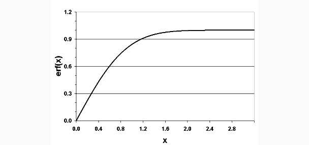
A very important function in the study of
Statistics is the Gaussian probability integral:
A slightly different relationship to erf(x) is more frequently seen in
mathematics:

The error function, erf(), is used in physics, engineering etc., to determine the
probability that events will occur between intervals of x. To determine values
for erf(x) we must evaluate the integral on the right of the expression.
(Excel2000 provides the
function ERF(z) but our aim is to demonstrate its calculation and provide a closed
form approximation for erf(). The steps of doing so provide further insight
into the use of the spreadsheet for one's own purposes.)
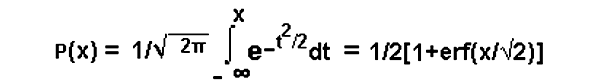
Gaussian Qradrature
Rectangular quadrature, representing the area of an interval
under a curve by the average of the start and finish values times the width of the
interval, works well when the curve is a straight line. If the curve could
be represented by an order two or higher polynomial, then other quadrature rules may produce better results.
In particular, the n-point
Gaussian Quadrature Rule can yield an exact result for polynomials of degree 2n-1.
The rule employs weighted values of the integrand at n points within the interval.
Points and weights for the interval from 1 to 2 for n = 4 are shown next.
Note that the abscissa labels are not proportionately
spaced.
Our calculation of erf(x) employs this 4 point Gaussian Quadrature Rule.
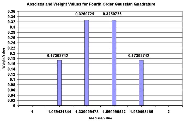
A plot of the integrand is shown next. It is a plot from columns B, for the abscissa,
and G, for the ordinate, of the spreadsheet that was used to calculate it.
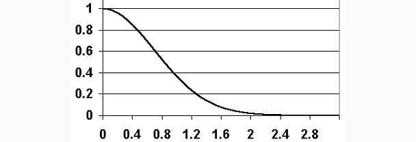
Representative cells from that spreadsheet now follow:
The expressions contained in the outlined cells can be seen by clicking their cell
addresses following:
|
E1
|
C2
|
E2
|
G2
|
I2
|
C3
|
|
D3
|
E3
|
F3
|
A6
|
B6
|
C6
|
|
D6
|
E6
|
F6
|
G6
|
H6
|
I6
|
Returning to the spreadsheet: Column A is for future use. Its values run from
zero to π/2 in steps of π/64000. Briefly, this column
will later serve as abscissa values for a sine series approximation to erf(x).
Column B values run from 0 to 3.2 in steps of 0.0001, (C1), and forms the intervals
of x for which the integrand is evaluated. The evaluations, (G6:G32005), employ the
value for e, (G1), and four points within each interval, as seen for (C6:f6),
using the weights shown at E1 and E2.
The incremental area, (H6), is formed as the product of the Gaussian Estimate of the
integrand times the width of the interval, (C1), times the multiplier 2/√π,
(I2).
The incremental areas are accumulated, summed, in column I to form the approximate erf(x)
which
is plotted from the table as is seen next.
How does it compare?
Using the same arguments, a table of the Excel2000 function ERF(x) was created
and the point-by-point relative difference, in %, between it and erf(x) was calculated
as ABS[(ERF(x)/erf(x)) -1]. The table is shown, in part, next.
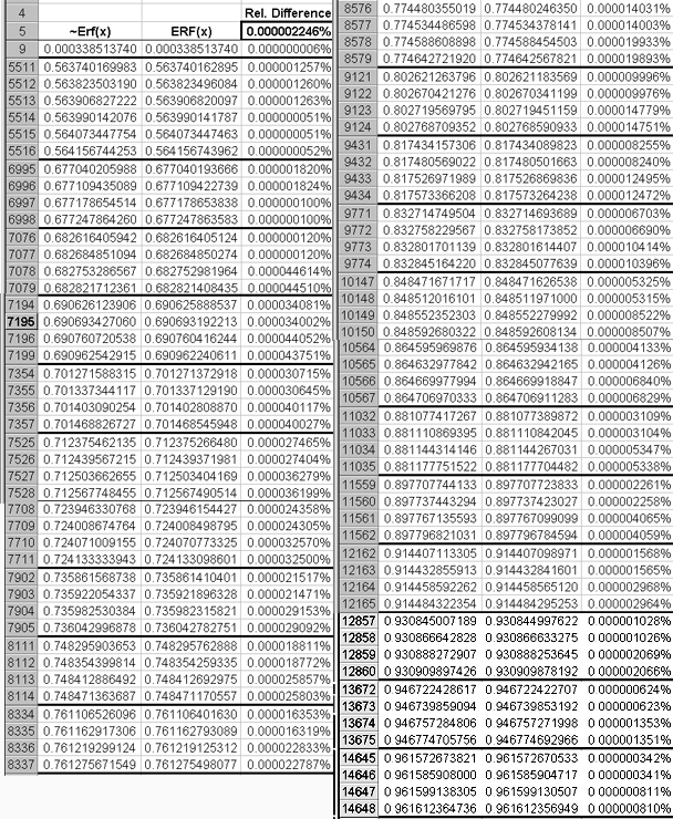
The average value of the relative differences is shown outlined at the top of the
third column.
Although less than half of the full table is shown, it is surmised from the
discontinuities, that ERF(x) is calculated in a sequence of ranges. For examples,
the first range finishes at row 5513; the second range finishes at row 6996; and
so on. A chart of the relative differences, which appear quite strange,
follows:
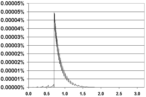
One wonders which of erf(x) or ERF(x) is the more accurate. Few values for
Erf() to be found on the web offer more than 7 decimal digits. IBM, at
this location, provides a 10 decimal digit value, 0.8427007794 for x = 1.
In comparison:
ERF(1) = 0.842700735175, differs from the IBM value by +0.000005248%. erf(1)
= 0.842700792950, differs from the IBM value by -0.000001608%, less than
1/3 of the relative difference provided by ERF(x).
As a second check:
"Computer Approximations",
The SIAM Series in Applied Mathematics, John Wiley & Sons, 1968
provides ARCERF(1/2) as 0.47693 62762 04469 87338 .....
. To compare without employing interpolation, the step size of the table,
0.0001
was modified slightly so that xo would assume this value quite closely, 0.47693627620449,
as is shown next at B4775 of the table.
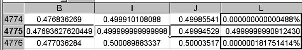
The corresponding value for erf() is shown at I4775 and
its series approximation at J4775. L4775 contains the Excel2000 value, ERF(B4775).
L4774 shows the relative error in percent of the table calculation with respect
to 1/2. L4776 shows the relative error of ERF(B4775).
Both of the foregoing tests against other known values serve to provide
more confidence in our spreadsheet table values than in the Excel2000 ERF() values.
Symmetry, Complement and Inverse
It is clear from the definition that erf(-x)
= erf(x). Note that the Excel2000 ERF(x) always expects a positive argument.
The complement of erf(x) is expressed as erfc(x) where erfc(x) = 1 - erf(x) and
is known as the error function complement. Excel2000 does not provide erfc(x).
The inverse of erf(x), the argument x of erf(x) for which erf(x) attains a specific
value, is expressed as arcerf(x). Excel2000 does not provide an ARCERF(x).
It can be obtained, approximately, by using their
Goal Seek tool from the Tools
menu as is illustrated next.
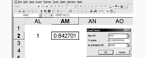
As seen in the foregoing, cell AL2 contains the value 1. As can be seen on the edit
line, cell AM2 contains the expression =ERF(AL2) and shows the appropriate value
in the cell. On selecting Goal Seek
from the Tools menu, the small menu
appears to allow entry of its parameters. Here we wish to change AL2 such
that AM2 will attain the value 1/3. Clicking OK brings up:
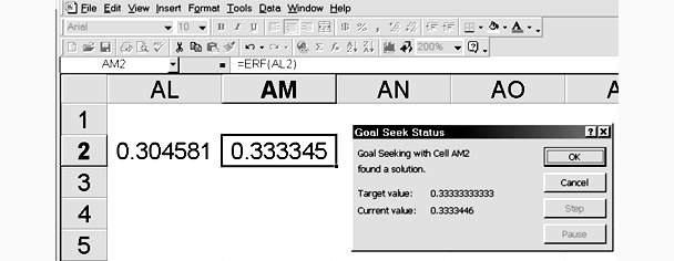
Although AM2 is not exactly 1/3, it is close. Writing one’s own macro can
provide a better approximation.
Goal Seek is quite a convenient
tool and worth knowing.
Approximate erf()
As it is time-consuming to look-up and interpolate in a table such as this,
it can be useful
to obtain an approximation for erf(x) that can be evaluated for
any x in the interval. The shape of the function suggests that a sine series could
be used
on the interval 0 to π/2 for the approximation as is seen next.
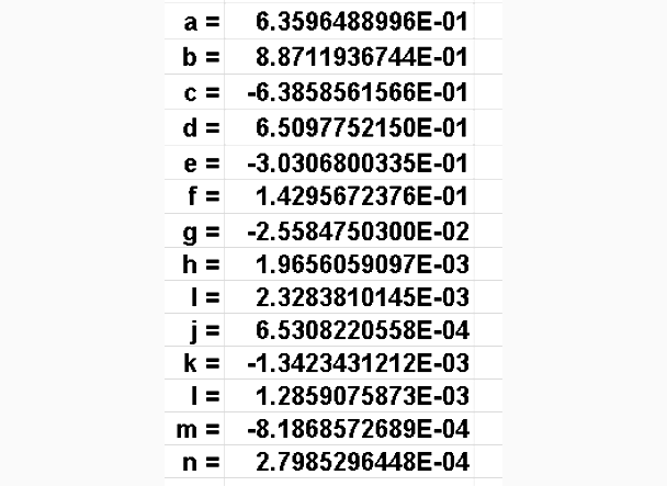
erf(u) = aSIN(u)+bSIN(2u)+cSIN(3u)+........+iSIN(12u)+mSIN(13u)+nSIN(14u)
Solver was used to find the coefficients a through
n using the average relative error between the calculated values
for erf(u) and the approximation as its objective function. The coefficients follow:
The sine series employs the variable u found in column A of the spreadsheet. Given
a value for x, u can be found as: u = π * x / 6.4.
A plot of the error between the approximation and the table follows:
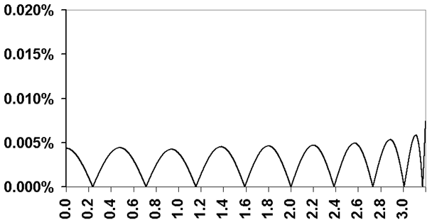
Note the almost uniform error extrema over the entire range of x. This effect
was produced by raising each relative error between erf() and its approximation
to the 12th power and using the average value of those errors as the objective function
for the approximation. What this does is greatly increase the influence of
large errors on the objective function, automatically providing them with more weight
and thus providing a larger target for minimization.
In many situations the
near uniform error extrema of relative error is a highly desirable feature of an
approximation.
As an exercise, the viewer might try to
improve on the approximation by approximating with functions other than the sine series.
A polynomial series or the ratio of two polynomial series could be tried.
The Normal or Gaussian Distribution
When the Gaussian probability integral employs
a density function that has a non-zero mean and has a non-standard width, t2
is replaced by (z-a)2 / 2σ2
where a is the average
or mean value of the density function and σ is a measure of its
width. The probability integral becomes:
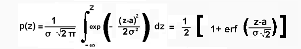
When
a is zero and
σ =1, p(z) regains its standard
normal form. See
here for further details.
Next
The next topic will employ the erf() function in a design problem.