Chapter 3
Grading Peas and the Central Limit Theorem
The inspiration for the treatment for this topic came
from an
abstract of "Seed Sizing with Image Analysis", a paper published by the
American Society of Agricultural
and Biological Engineers.
An excerpt from the abstract follows:
A flatbed scanner based image analysis application
was developed to size circular (peas), elliptical (soybean) and multifaceted (chickpeas)
shaped seeds by imaging a bulk poured sample. This application automatically separates
the seed boundaries in an image, measures individual seeds, and reports size distribution
for user-selectable sieve combination in metric or imperial units.
The image analysis equipment described foregoing is now presumed to be available
to a fictional company.
_____________________________________________
Some Fiction
Handson Food Processing Inc. is located in a large valley. The main agricultural
crop of the valley is green peas for human consumption. There are
many pea-producing
farms in the valley. Soils, farming practices, and weather
conditions are much the same for all the growers.
Although weather conditions and pea sizes vary from year to year, it has been found
over the years that about 25% of the crop are small enough to be packaged as their
Gourmet brand and about 15% of the crop are large enough to be used by their sister
company, Handson Soups Inc. The medium size, 60% of the crop, is packaged
as their Choice brand.
A variety of machines are used in pea processing. The hulls are removed by machine.
Stems, small stones, grit, dirt and chaff are removed using techniques such as flotation,
air blowers, vibration and screens. Some cleaning machines can be seen here.
The peas are all machine-harvested on a single day and placed in a chilled facility
for processing.
To determine the two needed size thresholds for the crop, a mixture of 30,000
peas taken equally from all of the different growers is analyzed and a binned size distribution is obtained for the mix. This season 44 bins were employed. The
bins are each
0.2 mm wide with centres ranging from 0.3 mm. through 8.9 mm. The average
size a and standard deviation Sigma of the sample
are shown on the chart of the distribution which is seen next.
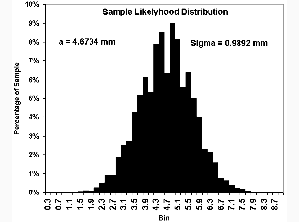
It does not appear easy to interpolate this binned distribution accurately,
to determine
the 25% and 85% size thresholds. A plot of the accumulated bin values
would serve better. See next.
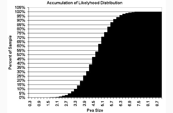
From this accumulation plot one could visually guess the 25% threshold as ~ 3.89
and the 85% as ~5.6.
If sieves were set up according to these values and the sample lot was processed,
20.81% would be classified as Gourmet peas and 17.38% would be classified as soup peas. Could
better thresholds be found?
Empiricism
Consider the human population of the state of Michigan. Within that population
consider the height of females ranging in age from 18 to 65 years. There are
about 3.75 million of these spread over 83 counties. Suppose now that you selected
400 of these females at random from each county, measured their heights, and calculated
the average height for the total selected. Would you expect this value
to be much different from those found for a second or third such random selection?
A similar question relates to a deviation from the mean. Some fraction of the
first selection are a centimetre or more taller than the mean height. Would
that fraction be much different for a second or third such selection?
Would you expect the fraction found in a selection, for those taller than the average
by two centimetres, to be smaller or larger than that found for those one centimetre taller?
Would you expect that such differences found between selections would become smaller
or larger
if the selections were made larger?
Answers to questions like these were first sought by carrying out experiments in
which aspects of large populations of beans, people, horse races, gambling games,
and the like were noted and analyzed, particular attention being given to obtaining
insight into possible strategies for making wagers.
Mathematics in Statistics
Empiricism was replaced by mathematical conclusions such as the formulation of
the Law of Large Numbers.
An excerpt from that reference follows:
The law of large numbers is a fundamental concept in statistics and probability that describes how the average of a randomly selected large
sample from a population is likely to be close
to the average of the whole population. The term "law of large numbers"
was introduced by
S.D. Poisson in 1835 as he discussed a 1713 version of it put forth by James Bernoulli
Another conclusion in mathematics, the Central
Limit Theorem, is
described here.
That description contains:
The central limit theorem is one of the most remarkable results of the theory of
probability. In its simplest form, the theorem states that the sum of a large number
of independent observations from the same distribution has, under certain general
conditions, an approximate normal distribution. Moreover, the approximation steadily
improves as the number of observations increases. The theorem is considered the
heart of probability theory, ....... .
A proof of the Central Limit Theorem can be seen
here.
Back to Pea Sorting
In accord with the Central Limit Theorem, we expect the pea sizes from the harvest
to have a Gaussian distribution.
A Gaussian distribution is entirely characterized by its mean and standard distribution.
Using a and Sigma
from the sample of peas, this distribution is plotted next.
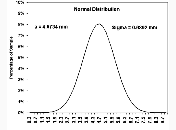 The foregoing plot is not necessary to our objective of
locating the two threshold
values and is shown here for interest only.
The foregoing plot is not necessary to our objective of
locating the two threshold
values and is shown here for interest only.
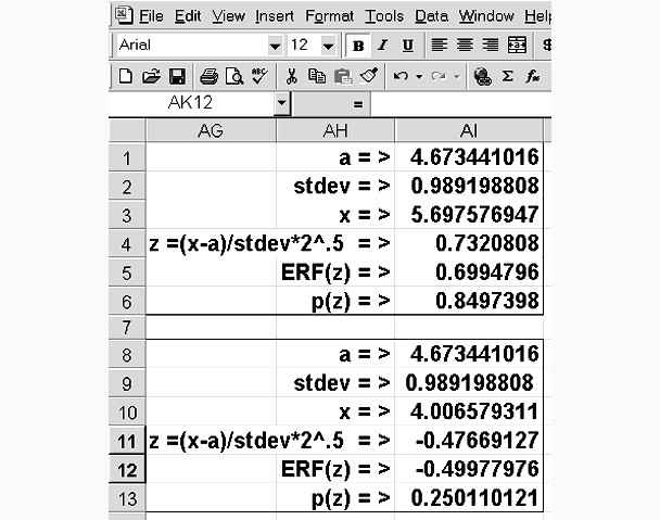
We could plot its accumulation and read its thresholds but it is
easier to employ ERF() that is also fully characterized by a and Sigma. See
a table for calculating a threshold next.
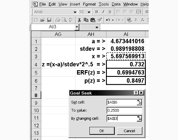
The expressions contained in the outlined cells can be seen by clicking their cell
addresses following:
The results of using Goal Seek for the two thresholds are shown next.
 (Had we wanted greater precision than that provided by Goal Seek, we could have
written a macro for the purpose.)
(Had we wanted greater precision than that provided by Goal Seek, we could have
written a macro for the purpose.)
Sieves were set up according to the threshold values 4.0 and 5.7 and the sample lot was processed. Now, 25.46% were classified as
Gourmet peas and 14.72% were classified as Soup peas.
Using the normal distribution as a proxy for the sample distribution to obtain the
thresholds provided a sorting result very much closer to the desired result than
did the thresholds obtained by estimation from the accumulation of the sample distribution.
_____________________________________________
Enough Fiction
The 30,000 samples of pea size that were the foundation of the processing story
were generated in accord with the teaching of the central limit theorem. There
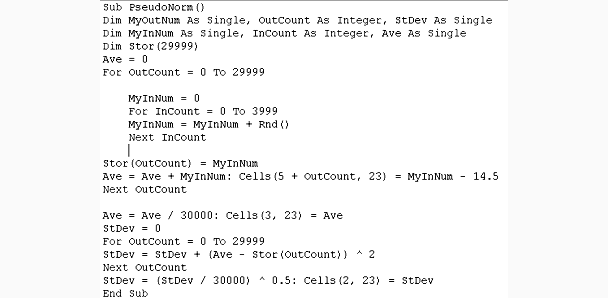
were two stages. First a small Excel2000 macro was designed to produce 30,000
pseudo random values. Then those values were scaled and shifted so as to have
a desired mean and standard deviation.
Excel's Visual Basic programming language provides a RND() function that generates
pseudo random values from zero up to but not including one. RND() is designed
to produce a uniform distribution on that interval, that is, all values produced
have the same likelihood of occurrence.
To construct each sample, 4,000 values from RND() were added together. The
central limit theorem teaches that such sums should tend to be normally distributed.
(The addition can be likened to 4000 stages in the growth of a pea.) Placing
30,000 of these sums on the spreadsheet together with the average sample value and
standard deviation completed the first stage. The macro follows:
A set of 30,000 values so produced should have an average value of ~2000.
This is a bit large for peas. Also, a standard deviation that could apply
to a pea crop was desired. Transforming these values to values suited to the
pea crop was accomplished by multiplying each of the samples by one selected constant
and adding another constant to the result. The objective values were a matter of mixed judgment,
trial and error, and not wanting the result to appear contrived.
The means of choosing the multiplier and additive constants may be interesting.
Excel's Solver add-in
can be used to choose parameters, the two constants, so as to set one value to a
desired value while
constraining other values. See the solver menu next.
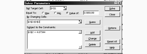
Here X1 is to be set equal
to the desired standard deviation by adjusting X3 and Y3, the desired constants,
subject to the constraint that X2 be the desired average value. (Solver
is a very
handy Excel tool.)
It may be of interest to see how some different sets of 30,000 samples produced
by the macro match in average value and standard deviation. These are shown
next for 5 consecutive sample sets.
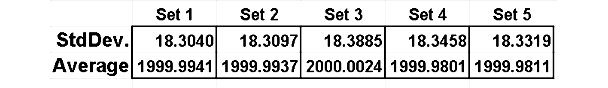
The Law of Large Numbers seems to be very well satisfied. The averages differ little
from their expected value of 2000.
Excel's Statistics Functions
Only one, NORMDIST(), of the about 80 available Excel2000 Statistics functions was
employed in this topic. It was used to generate the normal distribution plot
values for the bin abscissa given the sample
a and
Sigma.
Next
In the next topic, Numerical Integration and Interpolation
and some applications are explored.