Chapter 3
Using Accumulators for Integration -
Solving Some Differential Equations - Interpolating a List
A general purpose Integrator, based on Gaussian Quadrature
in conjunction with an accumulator, is described and applied to both calculating
some elementary math functions and to integrating an approximation.
Historical Integration
In the history of computing an integral there
have been many means employed for the integration.
Archimedes
found the area of an arc under a parabola, approximately, by summing terms of an infinite series.
The Planimeter has been used to determine
the area of two-dimensional shapes.
The Differential Analyser,
DA, employed a wheel and disk mechanism to perform integration.
The Op Amp Integrator was
based on the relationship between current and voltage of a capacitor and was a key
component of analogue computers.
Wikipedia describes the accumulator of a digital computer as:
In a computer's central processing unit, CPU,
an accumulator is a register in which intermediate arithmetic and logic results
are stored. Without a register like an accumulator, it would be necessary to write
the result of each calculation (addition, multiplication, shift, etc.) to main memory,
perhaps only to be read right back again for use in the next operation. Access to
main memory is slower than access to a register like the accumulator because the
technology used for the large main memory is slower (but cheaper) than that used
for a register.
The canonical example for accumulator use is summing a list of numbers. The accumulator
is initially set to zero, then each number in turn is added to the value in the
accumulator. Only when all numbers have been added is the result held in the accumulator
written to main memory or to another, non-accumulator, CPU register.
Integration employing an accumulator and
the series summation method of Archimedes have much in common.
A Spreadsheet Integrator applied to Squaring
Gaussian Quadrature was demonstrated in Topic 1 of this chapter as an integrating means to find the area under a curve. It is now characterized as a more general-purpose
integrator as will be described in conjunction with the spreadsheet table that
follows.

To view the cell expressions click a cell in the table following:
|
E1 |
E2 |
C3 |
D3 |
E3 |
F3 |
C4 |
D4 |
|
E4 |
F4 |
C7 |
D7 |
E7 |
F7 |
G7 |
H7 |
This spreadsheet table is very similar to that used to calculate erf(x)
in Topic
1. It employs 4-point Gaussian Quadrature to select the abscissas that are to be
used to represent the integrand in each integration interval.
A difference in this table is that the weights are combined with a constant K, at G1, to take into account any multiplier
of the integrand there may be. (In this table the integrand is a ramp function, 2 * x. Hence the value 2 was entered in cell G1.)
The Gaussian weights are calculated in E1:E2. The relative abscissas within
an interval are calculated in C3:F3. The weights accommodate K in C4:F4. The
actual abscissas to be employed for each interval are calculated in C7:F7. Accumulation
of the increments to the integral is accomplished by the expression
found in H7. The
cells of the spreadsheet, described foregoing, will remain the same for a variety
of integrands. Only the expression in G7 will be problem dependent.
The current expression in G7 is: =(C$4*C7+D$4*D7+E$4*E7+F$4*F7)*C$1 where C4:F4
are the weights given to evaluations of the integrand at the abscissas C7:F7.
(In this case, C7:F7 represent the current value of x.) C1 is the step size
i.e.,
width of the interval, and could have been incorporated into C4:F4 but has been
left here for clarity.
In many practical cases the integrand is a list of values rather than being in functional
form. This writer suggests that an approximation process be employed to fit
a function to the list values, much as was done in Topic 1 of this chapter in finding
a sine series fit to erf(z). Depending on the data set that is being
fitted, the underlying functions could be polynomials, ratios of polynomials, power
series, or sinusoids, among many other forms. The objective is a satisfactory
fit with a function that can be evaluated between listed values. A demonstration
of employing an approximation as an integrand will occur later in this topic.
The integrand, 2*x, of this example, as it represents a straight line, does not benefit from Gaussian quadrature.
What is illustrated in this example is the use of the accumulator for a solution
over a range of x, x = 0 to x = 3, of an ordinary differential equation
dy = 2*x dx.
That is, we use an accumulator to find y = x2
for a set of x values. The viewer should note that the squares are very precise,
and also that an initial value, 0 in H6, corresponding to x = 0, was provided to
the accumulator.
In
mathematics, an ordinary differential equation, ODE,
is a relation that contains functions of only one independent variable, and one
or more of its derivatives with respect to that variable.
ODEs arise in many contexts of science and engineering
including geometry,
mechanics, astronomy, physics and chemistry.
In the case where the equation is linear,
it can be solved by analytical methods. Most of the interesting differential
equations are non-linear and, with a few exceptions, cannot be solved exactly. Approximate
solutions are arrived at with the aid of computers.
A Spreadsheet Integrator applied to Calculating
the Natural
Logarithm
The spreadsheet table that follows is used for calculating LN(x) over the range
x = 1.02 to x = 4.02 at intervals of 0.02. This is accomplished by integrating
1/x.
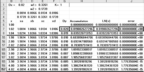
The essential differences between calculating LN(x) and x2
are:
now K = 1, and Dy, G7, has changed to reflect 1/x instead of x. Click the cell addresses,
next, to view the cell expressions.
Note that the initial value of the accumulator, H6, has been set to 0. Note
also the full agreement between the values in columns H and I.
An Approximation to a List of Values
The method of interpolating a list of values is to fit the list with an approximating
function. For an example list choose √0.5, √0.6, √0.7, √0.8, √0.9, √1.0.
As an interpolating, (approximating), function choose a ratio of two polynomials,
f(z) = (u1 +u2*z)/(v1+v2*z). Then employ Solver on a spreadsheet
to find suitable values for u1, u2, v1, and v2. An illustrating figure
follows:

The list is shown in column C of the Table. Initial values of 1 are provided for
u1:v2 at A2:B3. These produce a constant of 1 for f(z). See column B, and the line segment
plotted at 1 on the chart.
The absolute values of the relative errors between
list values and corresponding f(z) values is shown in column D. The sum of
those errors is shown in D3.
Solver, from the Tools Menu has been called to choose optimal values for u1:v2.
It has been set to adjust A2:B3 so as to minimize D3 with the six constraints, seen on Solver's menu, on
the relative errors. The effect of starting Solver by selecting
Solve is shown next.

Although the errors are now quite small, two are not as small as requested.
Higher order polynomials would fix this but we deem the result as close enough and
accept the solution.
Integrate the Approximation
The list has been converted from discrete values to a function, a ratio of two polynomials,
and is now suitable as an input to the spreadsheet integrator. That conversion is
analogous to the manual following of a plotted set of values on the input table
of a DA.
The six points of the list are square roots from the range x = 0.5 to x = 1.
It should be interesting to compare the integration of the functional approximation
to these points with the formal evaluation of the integral of y = √x for the same
range of x. This is done in the spreadsheet table seen next.

Expressions of the outlined cells can be seen by clicking their cell addresses in
the table following.
|
V7 |
W7 |
X7 |
Y7 |
Z7 |
AA7 |
AB7 |
AC7 |
Rather than carry out the evaluations of the function at the Gaussian sub-intervals
within the Dy column, four new columns for f(xa) through f(xd) have been inserted
for improved clarity. Their Gaussian weights are applied in column z,
Dy. The accumulator column AA, Acc., shows the increasing area under the
approximating function as x increases.
In column AB, Known, the integral from x = 0.5 to x = 1 of y =
√x is evaluated and is seen to closely match the values obtained by integrating
the approximating function.
The viewer may see applications with more rapidly varying integrands that
will require smaller step sizes to reach a desired precision than those employed in this
topic.
Conclusion
The spreadsheet integrator has been tested herein in three situations with extremely
good results.
A particular technique for interpolating tabulated values has been demonstrated.
There are many such. Of possible interest to the viewer, and not covered in Hands-On
Math, there could be Spline interpolation.
The viewer is urged to implement a spreadsheet integrator and explore its use.
Next
The next topic explores multiple numeric integration stages and error behavior.